07. Backpropagation
Backpropagation
Backpropagation
Now we've come to the problem of how to make a multilayer neural network learn. Before, we saw how to update weights with gradient descent. The backpropagation algorithm is just an extension of that, using the chain rule to find the error with the respect to the weights connecting the input layer to the hidden layer (for a two layer network).
To update the weights to hidden layers using gradient descent, you need to know how much error each of the hidden units contributed to the final output. Since the output of a layer is determined by the weights between layers, the error resulting from units is scaled by the weights going forward through the network. Since we know the error at the output, we can use the weights to work backwards to hidden layers.
For example, in the output layer, you have errors \delta^o_k attributed to each output unit k. Then, the error attributed to hidden unit j is the output errors, scaled by the weights between the output and hidden layers (and the gradient):
Then, the gradient descent step is the same as before, just with the new errors:
where w_{ij} are the weights between the inputs and hidden layer and x_i are input unit values. This form holds for however many layers there are. The weight steps are equal to the step size times the output error of the layer times the values of the inputs to that layer
Here, you get the output error, \delta_{output}, by propagating the errors backwards from higher layers. And the input values, V_{in} are the inputs to the layer, the hidden layer activations to the output unit for example.
Working through an example
Let's walk through the steps of calculating the weight updates for a simple two layer network. Suppose there are two input values, one hidden unit, and one output unit, with sigmoid activations on the hidden and output units. The following image depicts this network. (Note: the input values are shown as nodes at the bottom of the image, while the network's output value is shown as \hat y at the top. The inputs themselves do not count as a layer, which is why this is considered a two layer network.)
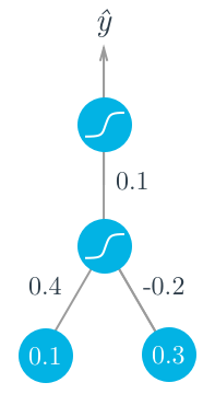
Assume we're trying to fit some binary data and the target is y = 1. We'll start with the forward pass, first calculating the input to the hidden unit
h = \sum_i w_i x_i = 0.1 \times 0.4 - 0.2 \times 0.3 = -0.02
and the output of the hidden unit
a = f(h) = \mathrm{sigmoid}(-0.02) = 0.495.
Using this as the input to the output unit, the output of the network is
\hat y = f(W \cdot a) = \mathrm{sigmoid}(0.1 \times 0.495) = 0.512.
With the network output, we can start the backwards pass to calculate the weight updates for both layers. Using the fact that for the sigmoid function f'(W \cdot a) = f(W \cdot a) (1 - f(W \cdot a)), the error term for the output unit is
\delta^o = (y - \hat y) f'(W \cdot a) = (1 - 0.512) \times 0.512 \times(1 - 0.512) = 0.122.
Now we need to calculate the error term for the hidden unit with backpropagation. Here we'll scale the error term from the output unit by the weight W connecting it to the hidden unit. For the hidden unit error term, \delta^h_j = \sum_k W_{jk} \delta^o_k f'(h_j), but since we have one hidden unit and one output unit, this is much simpler.
\delta^h = W \delta^o f'(h) = 0.1 \times 0.122 \times 0.495 \times (1 - 0.495) = 0.003
Now that we have the errors, we can calculate the gradient descent steps. The hidden to output weight step is the learning rate, times the output unit error, times the hidden unit activation value.
\Delta W = \eta \delta^o a = 0.5 \times 0.122 \times 0.495 = 0.0302
Then, for the input to hidden weights w_i, it's the learning rate times the hidden unit error, times the input values.
\Delta w_i = \eta \delta^h x_i = (0.5 \times 0.003 \times 0.1, 0.5 \times 0.003 \times 0.3) = (0.00015, 0.00045)
From this example, you can see one of the effects of using the sigmoid function for the activations. The maximum derivative of the sigmoid function is 0.25, so the errors in the output layer get reduced by at least 75%, and errors in the hidden layer are scaled down by at least 93.75%! You can see that if you have a lot of layers, using a sigmoid activation function will quickly reduce the weight steps to tiny values in layers near the input. This is known as the vanishing gradient problem. Later in the course you'll learn about other activation functions that perform better in this regard and are more commonly used in modern network architectures.
Implementing in NumPy
For the most part you have everything you need to implement backpropagation with NumPy.
However, previously we were only dealing with error terms from one unit. Now, in the weight update, we have to consider the error for each unit in the hidden layer, \delta_j:
\Delta w_{ij} = \eta \delta_j x_i
Firstly, there will likely be a different number of input and hidden units, so trying to multiply the errors and the inputs as row vectors will throw an error:
hidden_error*inputs
---------------------------------------------------------------------------
ValueError                                Traceback (most recent call last)
<ipython-input-22-3b59121cb809> in <module>()
----> 1 hidden_error*x

ValueError: operands could not be broadcast together with shapes (3,) (6,)
Also, w_{ij} is a matrix now, so the right side of the assignment must have the same shape as the left side. Luckily, NumPy takes care of this for us. If you multiply a row vector array with a column vector array, it will multiply the first element in the column by each element in the row vector and set that as the first row in a new 2D array. This continues for each element in the column vector, so you get a 2D array that has shape (len(column_vector), len(row_vector)).
hidden_error*inputs[:,None]
array([[ -8.24195994e-04,  -2.71771975e-04,   1.29713395e-03],
       [ -2.87777394e-04,  -9.48922722e-05,   4.52909055e-04],
       [  6.44605731e-04,   2.12553536e-04,  -1.01449168e-03],
       [  0.00000000e+00,   0.00000000e+00,  -0.00000000e+00],
       [  0.00000000e+00,   0.00000000e+00,  -0.00000000e+00],
       [  0.00000000e+00,   0.00000000e+00,  -0.00000000e+00]])
It turns out this is exactly how we want to calculate the weight update step. As before, if you have your inputs as a 2D array with one row, you can also do hidden_error*inputs.T, but that won't work if inputs is a 1D array.
Backpropagation exercise
Below, you'll implement the code to calculate one backpropagation update step for two sets of weights. I wrote the forward pass - your goal is to code the backward pass.
Things to do
- Calculate the network's output error.
- Calculate the output layer's error term.
- Use backpropagation to calculate the hidden layer's error term.
- Calculate the change in weights (the delta weights) that result from propagating the errors back through the network.
Start Quiz: